منبع : حمل
و نقل دریایی
کار عملی با نقشه های
دریایی
Plotting and piloting
Skip over navigation
Home Nav.
course Sailing Greece
Turkish Coasts
Yacht
charter Gulets


Lines of position
The modern chart shows us positions of many recognizable
aids to
navigation
like churches and lighthouses, which facilitate the approach to a
coastal area. This concept originated from a chart by Waghenaer and proved a milestone in the development of European
cartography. This work was called “Spieghel der Zeevaerdt”
and included coastal profiles and tidal information much like the
modern chart. It enables us to find the angle between the North and for
example an offshore platform, as seen from our position.
and proved a milestone in the development of European
cartography. This work was called “Spieghel der Zeevaerdt”
and included coastal profiles and tidal information much like the
modern chart. It enables us to find the angle between the North and for
example an offshore platform, as seen from our position.

Compass courses |

True courses |
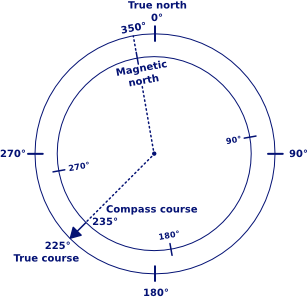
Taking a bearing on this oil rig with a compass provides
us with a compass course. This course first needs correction for both
variation and - via ship's heading - deviation before plotting a Line
of Position (LOP) in the chart as a true course.
Our
position is somewhere along this line.
Ranges
 A precise way to obtain a LOP, and without a compass, is to locate two
aids to navigation in line. The map of Laura Island on the right shows
four examples of ranges, each
consisting of two aids to navigation.
A precise way to obtain a LOP, and without a compass, is to locate two
aids to navigation in line. The map of Laura Island on the right shows
four examples of ranges, each
consisting of two aids to navigation.
Please, note that:
More distance between the two landmarks enhances
accuracy.
And less distance between the vessel and the closest aid
to navigation also enhances accuracy.
One of these four ranges consists of two lights that are
intentionally placed to provide a LOP. These pairs of lights are called
range lights or leading lights.
In this case they indicate the approach towards the marina and mark the
channel between the dangerous rocks along a true course of 50° . When looking towards any leading lights, the nearest one
will be lower.
. When looking towards any leading lights, the nearest one
will be lower.  Therefore, in the middle of the channel both lights will
appear vertically above each other.
Therefore, in the middle of the channel both lights will
appear vertically above each other.
Even when there are no man-made structures available, a
range can be found by using natural features such as coastlines and
islets. The example on the left shows a yacht that will avoid the
dangerous wreck as long as the islets don't overlap.
Position fix
If two LOPs intersect we can construct a position fix: the ship's position on the
earth.
Often
however, a triangle occurs when a third LOP is added in the
construction. This indicates that there are errors involved in at least
one of the bearings taken. In practice, we should consider each LOP as
the average bearing in a wider sector of for instance 10°.
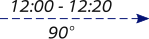
The optimum angular spread
is 90° (two objects) or 120°
(three objects). Moreover, bearings on distant objects bring about more
uncertainty in our position fix as the sector widens. Finally, if
moving fast you should not put any time between the bearings.
The next example features a nocturnal landfall on
Willemsen Island - you are welcome to visit, but mind the rocks. The
position fix is plotted by taking bearings at two light-vessels as their
lights appear over the horizon. The variation is -1° and the ship's compass heading is
190°. Since we use our steering compass for our bearings, we can use the same deviation table.
That means a deviation of -4° with which we can calculate (cc + var + dev = tc)
the true courses.
Construction

- Compass bearing
on Will. N is 72°
- True course is 67°
- Plot LOP with time & true course
- Compass bearing on Will. S is 173°
- True course is 168°
- Plot LOP with time & true course
- Draw an ellipse where the LOPs
intersect
- Notate time and “Fix”
alongside
- Position is 32° 04,2' N , 24° 46,7' E
|
|
Without a third LOP - forming the dreaded triangle -
there is the false suggestion of accuracy. Yet, instrument errors,
erroneous identification of an aid to navigation, sloppy plotting, etc.
can and will cause navigation errors. Therefore, if close to e.g. rocks,
you should assume to be at the worst possible position (i.e. closest to
the navigational hazard).
The lines plotted in the
chart are always true courses and these are labeled with true
courses by default; the “T” is optional. If labeled with the
corresponding magnetic
course or compass course add an “M” or “C”,
respectively.
Estimated position
It is sometimes impossible to obtain more than one LOP
at a time. To determine the ship's position with one aid to navigation
we can use a running
fix. However if a running fix is not possible, we can
determine an estimated position.
 An estimated position is based upon whatever incomplete navigational
information is available, such as a single LOP, a series of depth
measurements correlated to charted depths, or a visual observation of
the surroundings.
An estimated position is based upon whatever incomplete navigational
information is available, such as a single LOP, a series of depth
measurements correlated to charted depths, or a visual observation of
the surroundings.
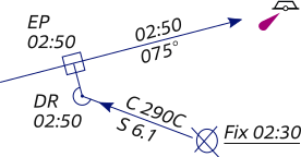
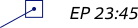
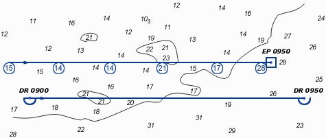
In the example on the right we see an estimated position
constructed using a single LOP and the ship's dead
reckoning position (DR).
This is done by drawing a line from the DR position at the time of the
LOP perpendicular to the LOP. An EP is denoted by a square instead of an
ellipse.
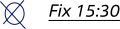
Do not rely on an EP as much as a fix. The scale of reliability, from best to worst:
Fix
Running fix
Estimated position
DR position
Dead reckoning
Dead reckoning
is a technique to determine a ship's approximate position by applying
to the last established charted position a vector or series of vectors
representing true courses and speed. This means that if we have an
earlier fix, we plot from that position our course and “distance
travelled since then” and deduce our current position.
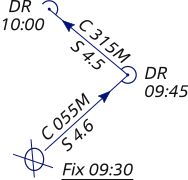
| 09:30 |
We start off with a Fix and plot a DR position for 15 minutes later. |
| 09:45 |
Our estimation about our speed and course was correct, so we don't
have to charge the DR position. |
| 10:00 |
and so on… |
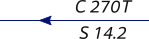
S = Speed through water (not over
ground)
C = Course through water (not over ground)
T = True
course (default)
M = Magnetic course for handheld compass
(no deviation correction)
C = Compass course for steering
compass (deviation correction)
Mark with an arrow, a semi-circle
(circular arc) and “DR”. | |
|
 |
Dead reckoning is crucial since it provides an
approximate position in the future. Each time a fix or running fix is
plotted, a vector representing the ordered course and speed originate
from it. The direction of this course
line represents the ship's course, and the length
represents the distance one would expect the ship to travel in a given
time. This extrapolation is used as a safety precaution: a predicted DR
position that will place the ship in water 1 metre deep should raise an
eyebrow…
In the example above the true courses are plotted in the
chart, and to assist the helmsman these course lines are labelled with
the corresponding compass courses.
Guidelines for dead
reckoning:
Plot a new course line from each new fix or running fix
(single LOP).
Never draw a new course line from an EP.
Plot a DR position every time course or speed changes.
Plot a corrected DR position if the predicted course
line proofed wrong, and continue from there.
Running fix
Under some circumstances, such as low visibility, only
one line of position can be obtained at a time. In this event, a line of
position obtained at an earlier time may be advanced to the time of the
later LOP. These two LOPs should not be parallel to each other;
remember that the optimal angular spread is 90°. The position obtained
is termed a running fix because the ship has “run” a certain distance
during the time interval between the two LOPs.
| 09:16 |
We obtain a single LOP on LANBY 1
and plot a corresponding (same time) dead reckoning position. The
estimated position is constructed by drawing the shortest line between
the DR and the LOP: perpendicular. |
| 09:26 |
No LOPs at all. We tack and plot a DR position. |
| 09:34 |
We obtain a LOP on LANBY 2. To use the first LOP we advance it over a
construction line between the two corresponding DR positions. We use
both its direction & distance. | |
|
 |
To use the LOP obtained at an earlier time, we must
advance it to the time of the second LOP. This is done by using the dead
reckoning plot. First, we measure the distance between the two DR
positions and draw a construction line,
which is parallel to a line connecting the two DR positions.
Note
that if there are no intervening course changes between the two DR
positions, it's easiest just to use the course line itself as the
construction line.
Now, using the parallel rulers we advance the
first LOP along this construction line over the distance we measured. Et
voilá, the intersection is our RFix.
If there is an intervening
course change, it appears to make our problem harder. Not so! The only
DR positions that matter are the two corresponding with the LOPs.
Guidelines
for advancing a LOP:
The distance: equal to the distance between the two
corresponding DR positions.
The direction: equal to the direction between the two
corresponding DR positions.
Draw the advanced LOP with a dotted line and mark with
both times.
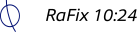
Label the Running Fix with an ellipse and "RFix"
without underlining.
Danger bearing
Like the dead reckoning positioning, the danger bearing
is an important tool to keep the ship out of harm's way. First, the navigator identifies the limits of safe, navigable water and
determines a bearing to for instance a major light. This bearing is
marked as “No More Than” (NMT) or “No Less
Than” (NLT), depending on which side is safe.
Hatching is included on the side that is hazardous, along with its
compass bearing.
First, the navigator identifies the limits of safe, navigable water and
determines a bearing to for instance a major light. This bearing is
marked as “No More Than” (NMT) or “No Less
Than” (NLT), depending on which side is safe.
Hatching is included on the side that is hazardous, along with its
compass bearing.
In the example on the right a true course of 325° is
plotted (5° variation), marked with the magnetic
course of 320°, practical for a handheld compass that
requires no deviation correction.
Were
we see that light at 350° magnetic - which is definitely “More Than” -
the rocks and wreck would be between us and the major light. A possible
cause could be a (tidal) stream from east to west.
When a distance is used instead of a direction, a danger range is plotted much the same way
as the danger bearing.
Turn bearing
The Turn bearing - like the
danger bearing - is
constructed in the chart in advance. It should be used as a means of
anticipation for sailing out of safe waters (again like the danger
bearing and dead reckoning). The turn bearing is taken on an appropriate
aid to navigation and is marked “TB”. As you
pass the object its bearing will slowly change. When it reaches the turn bearing turn the vessel on her new
course.
This type of bearing is also used for selecting an anchorage
position or diving position.
Snellius construction
Willebrord Snellius
- a 16th century mathematician from Leiden, the Netherlands - became
famous for inventing the loxodrome and his method of triangulation.
The
Snellius construction was first
used to obtain the length of the meridian by measuring the distance
between two Dutch cities.
He took angles from and to church towers of villages in between to
reach his objective. Nowadays we use the Snellius method to derive our
position from three bearings without the use of LOPs, and while leaving
out deviation and variation, which simplifies things. Also, since only
relative angles are needed a sextant can be used to measure navigation
aids at greater distances. Closer in a compass can be used.
The
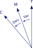
construction:
See figure 1: Compass bearings are 320° on A; 360° on
B; 050° on object C.
The angle between A and B = 40°.
The angle between B and C = 50°.
Draw lines from A to B and from B to C.
Add the two light-blue perpendicular bisectors of lines
AB and BC.
Draw at object A a construction line 40° inland of line
AB.
Draw at object C a second construction line 50° inland
of line CB.

See figure 2: At object A: draw a line perpendicular to
the construction line.
At object C: draw another line perpendicular to the
construction line.
The two intersections with the light-blue lines indicate
the centres of two circles.
Finally, draw the first circle using A and B and the
second circle using B and C.
The off shore intersection of the two circle gives us
our position fix.

The advantage: deviation and variation can be left out
since the angles (here 40° and 50°) are relative ones. Moreover, a
sextant can be used to obtain angles between objects at greater
distances, that with a compass would be less precise.
International notation
| International notation conventions for plotting
in the chart |
| Fix |
 |
|
LOP |
 |
| Running Fix |
 |
LOP advanced |
 |
| Estimated Position |
 |
Course & Speed |
 |
| Dead Reckoning |
 |
Set & Drift |
 |
| Electronic Fix (GPS) |
 |
|
|
| Electronic Fix (Radar) |
 |
|
|
Note, that a few countries use an alternative symbol 
Plotting should be done with a soft pencil. Moreover,
avoid drawing lines through the chart symbols. This is to prevent damage
to the chart when you have to erase the construction.
Learn sailing and
navigation via yacht charters with instruction in Greece.
Glossary
Line Of Position (LOP):
The
locus of points along which a ship's position must lie. A minimum of two
LOPs are necessary to establish a fix. It is standard practice to use
at least three LOPs when obtaining a fix, to guard against the
possibility of and, in some cases, remove ambiguity.
Transit fix: The
method of lining up charted objects to obtain an LOP.
Leading lights or Range lights: A pair of lights or day
marks deliberately placed to mark a narrow channel.
Position fix: The
intersection of various LOPs.
Cross bearing: The
use of LOPs of several navigational aids to obtain a position fix.
Remember to use an optimal angular spread.
Running fix: The
use of an
advanced LOP. Make sure to use only the corresponding DR positions. Also
don't use the EP for advancing the first LOP.
Dead reckoning:
Determining a
position by plotting courses and speeds from a known position. It is
also used to predict when lights become visible or to determine the set
and rate of a current.
Estimated position:
Combine a corresponding DR position with a single LOP to get an EP
position.
Snellius construction:
Another way to combine three compass bearings to obtain a position fix.
The advantage over a cross bearing is that both magnetic variation and
deviation don't need to be taken into account.
Course: (C) The
direction in which a vessel is steered or is intended to be steered
(direction through the water). Course to
steer: Course to steer to counteract current and leeway
[bovenstroomse koers].
 Heading (HDG):
The direction in which the boat is pointing in any instant
[voorliggende koers].
Heading (HDG):
The direction in which the boat is pointing in any instant
[voorliggende koers].
Course To Make Good
(CTMG): The course for planning purposes that indicates the
intended track from departure to destination.
Course Made Good (CMG): The single resultant direction
from the point of departure to the point of arrival at any given time.
Course line Construction line Danger range -->
Speed: (S) The
speed of the boat through the water. Speed
Made Good (SMG): The speed of the boat achieved over the CMG
line.
-->
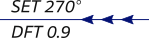
Set: (SET) The
direction in which the current is flowing (see chapters 6,7 and 8).
Drift: (DFT) The
speed (in knots) of the current (see chapters 6,7 and 8).
Default heading is
True course (M = magnetic , C = compass).
Default time is 24
hour clock ship time else UTC.
Piloting and
navigation
Skip over navigation
Home Nav.
course Sailing Greece
Turkish Coasts
Yacht
charter Gulets
Doubled angle fix
The Doubled angle on the
bow fix resembles a running fix though only one navigation aid
is used.
 |
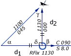
α = 30° , β = 60°
δ = 120° , γ = 30°
Isosceles
d1 = d2 |
In the example on the right the initial angle (30°) on
the bow is doubled (60°) yielding an isosceles triangle. The distance travelled between the bearings is the same as
the distance from the visible wreck.
Start with the visible wreck having a bearing of less
than 45° off the bow (α), note the log
distance.
Proceed along the course until the angle on the bow is
doubled (β), read the log: d1
is 10 nm.
Use the log distance to find the position on the second
LOP. It is an isosceles triangle, so d2 is also 10 nm.
Label it with an ellipse and "RFix" but realize
it is less precise than a running fix that involves two navigation
aids.
Four point fix
If the first angle on the bow is 45°, a special
situation occurs: The Four point fix,
so called since 45 degrees equals 4 points on the compass (1 point =
11,25°).
 |
α = 45° , β = 90°
δ = 90° , γ = 45°
Isosceles
d1 = d2 |
Start with a bearing with 45° on the bow (α),
note the log.
Proceed along the course till the angle on the bow is
90° (β), read the log: d1
is 4 nm
Use the log distance to find the position on the second
LOP. Isosceles, so d2 is also 4 nm.
Label it with an ellipse and "RFix".
Special angle fix
The Special angle fix
requires the mariner to know some special pairs of angles (a : b) that give
the distance travelled between bearings as equal to the distance abeam.
 |
α = 21° , β = 32°
d1
= d2 |
In the example on the right α =
21° and β = 32° are used. Now,
the log distance equals the shortest distance between wreck and course
line (6 nm).
A few practical pairs:
16 : 22 21 : 32
25 : 41 32 : 59
37
: 72 40 : 79
Remember: the greater the angular spread the better.
Hence, of these three fixes the four point fix is the most precise one.
Mathematics: isosceles triangle fixes
Distance of the horizon
On a flat world there would be no difference between the
visible and sensible horizon. However, on Earth the visible horizon appears several arc
minutes below the sensible horizon
due to two opposing effects: 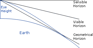
the curvature of the earth's surface;
atmospheric refraction.
Atmospheric refraction bends light rays passing along
the earth's surface toward the earth. Therefore, the geometrical horizon appears elevated, forming the visible horizon.
The
distance of the visible horizon is a (semi-empirical) function of Eye
Height:
Mathematics: horizon distances
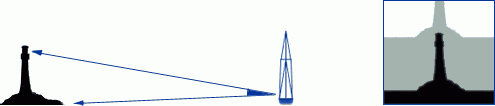
Dipping range
If an object is observed to be just rising above or just
dipping below the visible horizon, its distance can be readily
calculated using a simple formula.  The object's elevation (the
height of a light above chart datum)
can be found in the chart or other nautical publication such as the
'List of Lights'. Note that in some charts elevation is referred to a
different datum than soundings. Click on the image on the right to view a magnificent
lighthouse.
The object's elevation (the
height of a light above chart datum)
can be found in the chart or other nautical publication such as the
'List of Lights'. Note that in some charts elevation is referred to a
different datum than soundings. Click on the image on the right to view a magnificent
lighthouse.
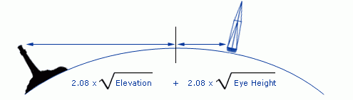
The formula contains the two distances from the visible
horizon and can be simplified by the equation: 2.08 x (√Elevation + √Eye
height). Many nautical publications contain a table
called "distances of the horizon" which can be used instead of the
equation.
Use the dipping range to plot a Distance LOP
in the chart: a circle equal in radius to the measured distance, which
is plotted about the navigation aid. Finally, take a bearing on the
object to get a second LOP and a position fix.
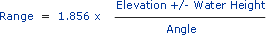
Vertical sextant angle
Similarly, a distance LOP can be obtained by using a
sextant to measure the angle (arc) between for instance the light and chart datum of a lighthouse or any other structure of
known elevation. Once the angle is corrected for index error the distance can be found in a
table called: "Distances by Vertical Sextant Angle", which is based on
the following equation.
The angle in minutes total, thus 1° 12' = 72' total, and
corrected for index error.
Elevation in metres.
Water height in metres above or below chart datum of
object.
Distance or Range in nautical miles.
Ascertain whether the base of the object is beyond the
horizon
Corrected angle should be greater than 20'.
Though tables can be used for quick reference, this
function is valid for objects higher than usually tabulated. An example with a lighthouse of 80 metres:
Measured angle is 1° 19', index error is +6': angle =
73'.
Let's assume water height at 3 metres above Mean Level
datum.
Range = 1.854*(80-3/73) = 1.96 nm.
The range can be used as a danger bearing.
Together
with a compass bearing one object with known elevation results in a
position fix. If more than one vertical sextant angle is combined the
optimum angular spread should be maintained.
Often, the correction for water height
can be left out. Though, realizing that the horizon is closer than one
might think,
another correction is sometimes needed. In the Mediterranean Sea for
example we can see mountain tops with bases lying well beyond the
horizon. Mutatis mutandis, the structures, which they bear have bases
beyond the horizon as well.
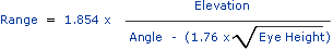
This is the equation for finding the distance of an
object of known elevation located beyond the horizon. In the denominator
of this equation a compensating factor is included by which the
measured angle should be reduced.
Mathematics: vertical sextant angles
Estimation of distance
The most obvious way to estimate distances is of course
by using the distance between our eyes.  If we sight over our thumb first with one eye then with the other, the
thumb moves across the background, perhaps first crossing a tower second
crossing a bridge.
If we sight over our thumb first with one eye then with the other, the
thumb moves across the background, perhaps first crossing a tower second
crossing a bridge.
The chart might tell that these structures are 300 m
apart.
Use the ratio of: distance between eye and outstretched
arm/distance between pupils: usually 10.
The objects are 3 kilometres away.
Other
physical relationships are useful for quick reference. For example, one
finger width held at arm's length covers about 2° arc, measured
horizontally or vertically.
Two fingers cover 4°. Three fingers cover
6° and give rise to the three finger rule:
"An
object that is three fingers high is about 10 times as far away as it
is high."
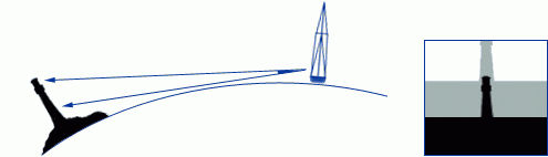
Estimation with horizon
The image on the right shows us that it is possible to
estimate the height of any object that crosses the horizon as seen from
our own point of view.
This picture of the 'Pigeon Rocks' near Beirut harbour
was taken from a crow's nest at a height of 34 metres.
The distance
of the visible horizon (12 nm) is far larger than 34 metres. Therefore, we can - without any other information -
estimate that these rocks have a height of 34 metres as well.
Factum: All tops crossing the horizon
and with bases at sea level are on eye level.
Furthermore, if we see these rocks over a vertical angle
of for example 7° = 0.1225 rad., then the range is
34/0.1225 = 277 metres.
Finally, plot both range and bearing in the
chart to construct an EP, et Voilà!
Fix by depth soundings
A series of depth soundings - in this example every 10
minutes - can greatly improve your position fix:
correct your soundings for tide, etc.;
copy the DR course line on a transparent sheet;
write the depths adjacent according to the times of the
soundings;
move the sheet over the chart to find its best location.
Due to leeway, currents or other factors the two course
lines need not be parallel to or of same length as each other.
Yacht charters and
learning how to sail in Greece with instruction.
Overview
Line Of Position (LOP):
The
locus of points along which a ship's position must lie. A minimum of two
LOP's are necessary to establish a fix. It is standard practice to use
at least three LOP's when obtaining a fix, to guard against the
possibility of and, in some cases, remove ambiguity.
Range or Distance LOP:
Obtained by using a stadimeter, sextant or radar. A circle equal in
radius to the measured distance is plotted about the navigation aid; the
ship must be somewhere on this circle.
Running fix: A
position determined by crossing lines of position obtained at different
times and advanced or retired to a common time.
Dead reckoning:
Determining a
position by plotting courses and speeds from a known position. It is
also used to predict when lights become visible or to determine the set
and drift of a current. DR positions are drawn in advance to prevent
sailing into danger. A DR position will be plotted:
-
every hour on the hour;
-
at the time of every course change or speed change;
-
for the time at which a (running) fix is obtained,
also a new course line will be plotted;
-
for the time at which a single LOP is obtained;
-
and never draw a new course line from an EP position!
Estimated position:
The most
probable position of a craft determined from incomplete data or data of
questionable accuracy. Such a position might be determined by applying a
correction to the dead reckoning position, as for estimated current; by
plotting a line of soundings; or by plotting a LOP of questionable
accuracy.
Double angle on the bow:
A
method of obtaining a running fix by measuring the distance a vessel
travels on a steady course while the relative bearing (right or left) of
a fixed object doubles. The distance from the object at the time of the
second bearing is equal to the run between bearings, neglecting drift.
Four point fix: A
special
case of doubling the angle on the bow, in which the first bearing is 45°
right or left of the bow. Due to angular spread this is the most
precise isosceles fix.
Special angle fix:
A
construction using special pairs of relative angles that give the
distance travelled between bearings as equal to the navigation aids'
range abeam.
Distance from horizon:
The distance measured along the line of sight from a position above the
surface of the earth to the visible horizon.
Sensible horizon:
The circle
of the celestial sphere formed by the intersection of the celestial
sphere and a plane through the eye of the observer, and perpendicular to
the zenith-nadir line.
Visible horizon:
The line
where Earth and sky appear to meet. If there were no terrestrial
refraction, visible and geometrical horizons would coincide. Also called
: apparent horizon.
Geometrical horizon:
Originally, the celestial horizon; now more commonly the intersection of
the celestial sphere and an infinite number of straight lines tangent
to the earth's surface and radiating from the eye of the observer.
Dipping range or Geographic range:
The maximum distance at which the curvature of the earth and
terrestrial refraction permit an aid to navigation to be seen from a
particular height of eye (without regard to the luminous intensity of
the light).
Elevation: The
height of the light above its chart datum in contrast to the height of
the structure itself.
Chart Datum:
Officially:
Chart Sounding Datum: An arbitrary reference plane to which both heights
of tides and water depths are expressed on a chart. In the same chart
heights can be related to other datums than depths.
Vertical sextant angle:
The method of using the subtended angle of a vertical object to find
its range.
Index error: In a
marine
sextant the index error is primarily due to lack of parallelism of the
index mirror and the horizon glass at zero reading. A positive index
error is subtracted and a negative index error is added.
Estimation with horizon:
Estimation of heights using the horizon: All tops crossing the horizon
and with bases at sea level are on eye level.
Estimation
with depth effect: .
Estimated
position with soundings:
 2011 update at 19-10-2011

 Featuring
two highs and two lows each day, with minimal variation in the height
of successive high or low waters. This type is more likely to occur when
the moon is over the equator.
Featuring
two highs and two lows each day, with minimal variation in the height
of successive high or low waters. This type is more likely to occur when
the moon is over the equator.  Only
a single high and a single low during each tidal day; successive high
and low waters do not vary by a great deal. This tends to occur in
certain areas when the moon is at its furthest from the equator.
Only
a single high and a single low during each tidal day; successive high
and low waters do not vary by a great deal. This tends to occur in
certain areas when the moon is at its furthest from the equator.  To
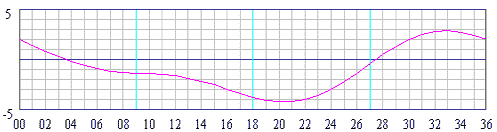
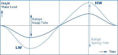
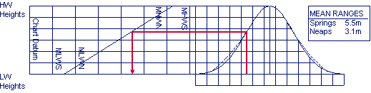
interpolate between high and low water heights we use the Rule of Twelve.
We assume the tidal curve to be a perfect sinusoid with a period of 12
hours. The height changes over the full range in the six hours between
HW and LW.
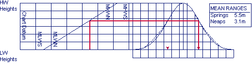
To
interpolate between high and low water heights we use the Rule of Twelve.
We assume the tidal curve to be a perfect sinusoid with a period of 12
hours. The height changes over the full range in the six hours between
HW and LW. 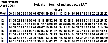 provides us each day with the times of high and low water for a
particular place. Basically, it is same table like the one we found in
the chart, but is extended for every day in a year. By using this method
we get more accurate water heights since it involves less
interpolation. The example shows us a part of a very detailed tide
table, which even includes heights for every hour.
provides us each day with the times of high and low water for a
particular place. Basically, it is same table like the one we found in
the chart, but is extended for every day in a year. By using this method
we get more accurate water heights since it involves less
interpolation. The example shows us a part of a very detailed tide
table, which even includes heights for every hour. 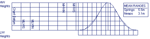


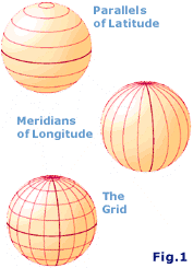 that covers our planet with
imaginary lines called meridians
and parallels, see figure 1. All
these lines together provide the grid which enables us to describe any
position in longitudes and latitudes.
that covers our planet with
imaginary lines called meridians
and parallels, see figure 1. All
these lines together provide the grid which enables us to describe any
position in longitudes and latitudes. 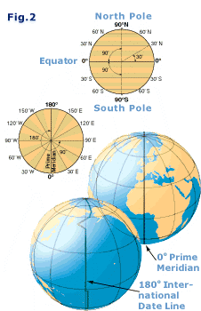 The North Pole has a latitude of 90° N and the South Pole
90° S. The meridians cover twice this angle up to 180° W or E.
The North Pole has a latitude of 90° N and the South Pole
90° S. The meridians cover twice this angle up to 180° W or E.  into
360 degrees, or 360° x 60' = 21600' minutes. In 1929, the international
community agreed on the definition of 1 international nautical mile as
1852 metres, which is roughly the average length of one minute
of latitude i.e. one minute of arc along a line of longitude (a
meridian).
into
360 degrees, or 360° x 60' = 21600' minutes. In 1929, the international
community agreed on the definition of 1 international nautical mile as
1852 metres, which is roughly the average length of one minute
of latitude i.e. one minute of arc along a line of longitude (a
meridian). 
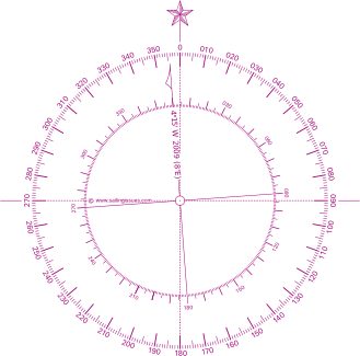
 These overlayed compass roses show the difference between true north
and magnetic north when the magnetic variation is 10° West.
These overlayed compass roses show the difference between true north
and magnetic north when the magnetic variation is 10° West.